Taking the First Steps into the World of Probability

Benjamin Chen
2022年1月27日
讀畢需時 9 分鐘

已更新：2024年1月22日

Probability is a huge headache to many people, and it’s totally understandable. When probabilities become more complicated, people struggle to visualize the imaginary pie that we’re all used to thinking. This story will try to break down the basics of probability and give you visualizations that will allow you to understand different types of probability. But before we begin, we must clarify the meaning of several crucial terminologies.

Outcome – the results of an experiment
Event – set of outcomes to which a probability is assigned
Sample Space – a collection of all possible outcomes

The difference between the three terms can be clearly illustrated by a dice-rolling example. When we roll some dice, the six possible outcomes are 1, 2, 3, 4, 5 and 6. The collection of these six numbers is my sample space. An event, on the other hand, could be “rolling a number that is less than 3”, which has a probability assigned to it (and we all know it is 2/6). There are two types of events that we will discuss here, a simple event and a joint event.

Simple Event – an event described by one characteristic
Joint Event – an event described by two or more characteristics

Let’s also differentiate the two types of events using an example. A simple event could refer to a student who is majoring in Accountancy. A joint event, on the other hand, could refer to a student who is not only majoring in Accountancy but also a freshman (described by two conditions).

Finally, we have the complement of an event. The complement of an event refers to all events that are not part of the event. If event A is selecting a student majoring in Accountancy, then the complement of Event A would be selecting a student not majoring in Accountancy (so a student in every other major).

Contingency Table and Decision Tree

Contingency Table

To facilitate the calculation of probability, data are often visualized in either form of contingency tables or decision trees. A contingency table displays the frequency distribution (count) of the variables used. Look at the example below:

Here, we have a contingency table for a deck of cards. The contingency table is composed of two variables, Ace or Other (first row) and Black or Red (first column). We can see how the 52 cards in a deck are distributed across these two variables into their corresponding cell. The 2 in the first cell means only 2 cards are both Ace and Black (Ace of Spades and Ace of Clubs). You can verify the other numbers as well.

Decision Tree

A decision tree is much like a contingency table but formatted in a different way. Taking the same example on a deck of cards, the decision tree would look like this:

The decision tree branches off and the frequency distribution is listed at the end of each branch.

We will repeatedly come back to these visualizations, especially the contingency table, to illustrate probabilities, so it’s important you know how to read them. Anyways, let’s actually start talking about probability.

Probability

A probability is a numerical value representing the possibility that a particular event will occur. The probability of an event is always between 0 and 1 (inclusive).

Notation for the probability of event A:

If an event is certain (100% chance of occurrence), then the probability of the event is 1. If an event is impossible (0% chance of occurrence), then the probability of the event is 0.

The Three Ways of Assessing Probability

There are three ways to assess probability:

1. Prior

2. Empirical

3. Subjective

The prior way assesses probability based on ‘prior’ knowledge of the process. So, if we were to toss a coin, the prior probability of tossing a head would be 0.5. This is because based on our ‘prior’ knowledge that a coin has two sides and is congruent, we assign equal probabilities to each side.

The empirical way assesses probability based on actual experimentation. So for the same coin-tossing example, to obtain the empirical probability of tossing a head, we would need to carry out the experiment. Say we obtained 515 heads out of 1000 tosses for our experiment, our empirical probability of landing a head would then be 0.515.

The subjective way of assessing probability is simply based on an individual’s experience, opinion and analysis of the situation.

Joint and Marginal Probability

Next, let’s introduce the types of probability. We have joint probabilities and marginal probabilities. A joint probability is the probability of a joint event, and a marginal probability is the probability of a simple event. Let’s visualize these two probabilities with a contingency table.

Here we have a contingency table of the two variables “Planned to Purchase” and “Actually Purchased”.

An example of a joint probability would be the probability of someone who planned to purchase AND actually purchased. From the contingency table, we can see that 200 people (out of the 1000 people in the table) fall into this cell. That means this joint probability is 200/1000.

An example of a marginal probability would be the probability of someone who didn’t plan to purchase. From the contingency table, we can see that 750 people (out of 1000) didn’t make any plans to purchase. That means this marginal probability is 750/100.

You might have also realized that we can calculate this marginal probability by adding 100/1000 and 650/1000.

In fact, the marginal probability is the sum of the probability of X=x for all outcomes of y, given that y events are mutually exclusive and collectively exhaustive.

Ok, that was a difficult statement to comprehend. Let’s break this sentence down.

In our contingency table, we have two variables, “Planned to Purchase” and “Actually Purchased”. We can refer to these two variables as our X and Y variables. The values for the X and Y variables are denoted in lowercase x and y. So, if “Planned to Purchase” is the X variable, “Yes” and “No” are the possible x values.

Now, remember that our marginal probability can be calculated by adding 100/1000 and 650/1000.

The 100/1000 is the joint probability of someone who didn’t plan to purchase AND actually purchased. The 650/1000 is the joint probability of someone who also didn’t plan to purchase AND didn’t actually purchase. “Actually Purchase” and “Didn’t Actually Purchase” are all the outcomes of y. So the marginal probability of someone who didn’t plan to purchase (Planned to purchase = No) would be the sum of the probability of Planned to purchase = No for all outcomes of y.

But don’t forget there’s a second part to that statement, “given y events are mutually exclusive and collectively exhaustive”. Let’s define these two terms first.

Mutually Exclusive and Collectively Exhaustive

When we describe events as mutually exclusive, these events will never occur simultaneously. For example, we would describe the event of picking a diamond from a deck of cards and the event of picking a heart from a deck of cards as mutually exclusive. It is impossible to pick a card that is both diamond and heart.

When we describe events as collectively exhaustive, these events cover the entire sample space. If we use the same example, picking a diamond and heart from a deck of cards, the two events are not collectively exhaustive. Diamonds and hearts do not cover the entire sample space. The two card types only account for half of an entire deck. If the events were selecting a black card and selecting a red card, then these two events would be collectively exhaustive. All cards must be in one of the two colors.

Now let’s come back to our statement.

The marginal probability is the sum of the probability of X=x for all outcomes of y, given that y events are mutually exclusive and collectively exhaustive.

In the context of our example, the latter condition becomes “given ‘Actually Purchased’ and ‘Didn’t Actually Purchased’ are mutually exclusive and collectively exhaustive”. This condition is crucial because if the y events weren’t mutually exclusive (y events could occur simultaneously), there’s a chance you could double count probability when calculating the marginal probability. On the other hand, if y events weren’t collectively exhaustive (y events do not cover all sample space), there’s a chance you could miss count probability when calculating the marginal probability.

Ok, let that sink in! Perhaps, it’s not the smartest to spend this much time and effort on this one statement. But it’s important to understand these properties and conditions, particularly the concept of mutually exclusive and collectively exhaustive. This concept will stick with us along many topics of statistics.

Next, let’s discuss some more complicated forms of probability.

General Addition Rule

The general addition rule is the formula to find the probability of event A OR event B. The formula looks like this:

Now, you can just memorize this formula and apply it whenever needed, but let’s try to understand the composition. Once you understand what this formula means, you will never need to memorize it again. But first, let’s clarify the difference between OR and AND.

OR means that the outcome has to satisfy at least one condition.
AND means the outcome has to satisfy both conditions.

Coming back to our purchasing example, the probability that someone planned to purchase OR actually purchased will be 350/1000 (in orange). You can see that the people in these three cells satisfy at least one of the two conditions.

Now we can break down the general addition rule.

If we apply the equation to our example, the equation will look like this:

Let’s first identify P(Planned to Purchase) in blue and P(Actually Purchased) in red.

You can see that if we add these two probabilities together (300/1000 + 250/1000), we get 550/1000. This is 200/1000 higher than the correct answer (we previously identified the probability as 350/1000). This is because we counted their joint probability, P(Planned to Purchase AND Actually Purchased), twice when we summed up the two probabilities. I circled the double-counted probability in green for you to identify. That is why at the end of the equation, we must deduct the two events’ joint probability, so we don’t double count.

In cases where the two events are mutually exclusive (cannot occur simultaneously), the general addition rule can be simplified to just:

This shouldn’t be too hard to understand because when eg. event A and event B are mutually exclusive, their joint probability, P(A and B), is 0. So we can remove the latter part of the equation.

Conditional Probability

Next, let’s talk about conditional probability. Conditional probability is the probability of one event given another event. The notation of conditional probability is illustrated below.

The notation is read as the probability of event A given event B. The formula for conditional probability is:

Again, you can choose to memorize this formula, but let’s visualize this so we can truly understand conditional probability. Consider rolling six-sided dice. We have six possible outcomes, 1-6, when we throw some dice.

Say we want to find the probability of landing an even number given it is less than 4. Let’s first follow the formula without giving in any thoughts.

The answer is 1/3. Now let’s try to visualize this formula. By the formula, we can see that the “given”, less than 4, is the denominator. That means we are limiting our outcomes to those that only satisfy the “given” condition. In our example, our “given” is a number that is less than four. Let’s mark those out in green.

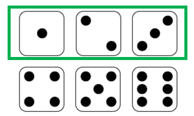
Only these three outcomes satisfy our “given” condition. Now, we can come back to see the probability that we want to find, landing an even number. Out of the three outcomes that satisfy our “given” condition, only number 2, is an even number (marked in purple).

We can see that the probability of landing an even number given the number is less than 4 is 1/3, and this is congruent with the result we used from the formula. Get it now? Conditional probability is actually super simple!

Now let’s come back to our formula once again.

If we move the denominator to the left side of the equation, we can derive:

This new equation is also called the general multiplication rule. It might come in handy when you are asked to calculate a joint probability P(A and B).

Statistical Independence

Alright! Next comes a very very very important topic, statistical independence! This is something you will consistently encounter throughout your statistics career, so be sure to understand this. If event A and B are independent, that means event A will not affect the probability of event B, and vice versa. In notation, we can write the following:

Despite including the condition of event B, the probability of event A remains the same. Let’s visualize statistical independence with a contingency table. Assume the pet as the A variable and gender as the B variable.

You can see that out of the 100 people surveyed, 51 voted for a dog, and 49 voted for a cat.

But if I focus on just the male responses, we can see that out of 52 male responders, 42 voted for a dog and only 10 voted for a cat.

Before we included the male condition, the probability of voting for a dog was only 0.51. After we included the male condition, the probability of voting for a dog increased up to 0.808. Recall the notation for statistical independence.

In our example, the notation would become:

And we can see that the notation does not apply in our example because:

This means event dog and event male are not statistically independent. Whether or not the responder is a male does affect the preference over dogs. Get it now? The shortcut way to check statistical independence is just to check whether the notation (below) applies. If it does, then the two events are independent. If it doesn’t, then the two events are dependent.

Conclusion

Hooray! We are done with probability! We covered quite a lot of topics, so let's do a brief recap:

Contingency Table and Decision Tree
Three Ways of Assessing Probability
Marginal Probability and Joint Probability
Mutually Exclusive and Collectively Exhaustive
General Addition Rule
Conditional Probability
General Multiplication Rule
Statistical Independence

We will return to some of these concepts in the future, so make sure you go through these thoroughly. In our next story, we will go over 5 useful counting rules that will make your life much easier.