Exploring the Differences: A Comparison of Two Population Means

In the last story, we compared two proportions and performed CI estimation and hypothesis testing to see whether the difference in proportion is significant. In this story, we will proceed with our discussion on the comparison of two means. Given two distributions of sample means, characterized by different categorical variables (explanatory), how could we properly compare the two to see if there is a statistical difference?

First, for comparing sample means, we have to consider whether the two populations are independent. The samples from two populations are independent if the samples from one population have no relationship with the samples in the other population. On the other hand, samples are dependent if a sample seems to appear in both populations. Let's take a look at an example to differentiate the two.

Independent:

Say we are interested in evaluating the gas mileage of two brands of gasoline. The samples are independent if we assign 10 cars to brand A and another 10 cars to brand B. The samples of the two brands are not related to each other.

Dependent:

The samples would become dependent if we assign 10 cars to use both brand A and brand B subsequently. The samples in two brands can be matched or "paired". This is why dependent samples are also called paired data.

Depending on whether the samples are independent between the populations, we would approach our objective of comparing the two means slightly differently. Let's start by looking at the cases where samples between populations are independent.

---

Inference for Independent Means

You should recall from Statistics 9: Sampling Distribution Clearly Explained! that, given the population is normal or that sample size is large enough (n>=30), sample means typically follow:

Note: When the population standard deviation is unknown, it is replaced by the sample standard deviation.

Going back to the last story on comparing two population proportions, we also learned that we could apply the following theory to find the difference between two normally distributed distributions:

Therefore, in the case of finding the difference between two sample means, we can say that:

This is where things get a little tricky. Looking at the formula above, we know that the two population standard deviations are usually unknown. It's natural to think that we could simply substitute them with the sample standard deviations. While this is the typical practice, the estimates may not be that accurate, especially when the sample size is small. Instead, it would probably lead to a better estimate by using the common standard deviation, derived from pooling the data from both populations. But be careful! This approach should only be used when the standard deviations for the two populations are not that different. We'll take a more detailed look into this approach later in this story.

Ok, let's quickly summarize the flow map for comparing two means!

First, we determine whether the two samples are independent. If they are independent, we then have to check whether to two populations have similar standard deviation (or variance). That will then decide whether we should use a pooled variance or an unpooled variance.

---

Pooled Variance

Let's first assume that the two populations do have similar standard deviations and that we should estimate the common variance by pooling the data from both populations. Note that it is often ambiguous to tell to what extent is 'similar' standard deviations similar enough. We will go through a statistical test later to see how we can properly determine if two standard deviation is significantly different. For now, let's just assume that they're close enough.

Now that we have two samples extracted from two populations, we would be able to calculate two sample means and two sample standard deviations.

Using these notations, we can calculate the pooled standard deviation by using the following formula:

We can use this as the new estimate for the unknown population standard deviation, and thus the formula for the t-test statistics would become:

Again, remember that this formula is given under the assumption that the two populations are independent, normal or have a large sample size, and has a fairly similar variance (or standard deviation). The t-statistics will follow a t-distribution with n1 + n2 - 2 degrees of freedom.

Confidence Interval

We can also now derive the formula for our confidence interval for mu1 - mu2.

Example

Now let's apply what we just learned about comparing two means using the pooled variance in an example. This example is extracted from Penn State Stats Online.

In a packing plant, a machine packs cartons with jars. It is supposed that a new machine will pack faster on average than the machine currently used. To test that hypothesis, the times it takes each machine to pack ten cartons are recorded. The results, in seconds, are shown in the tables.

New Machine	42.1	41.3	42.4	43.2	41.8	41.0	41.8	42.8	42.3	42.7
Old Machine	42.7	43.8	42.5	43.1	44.0	43.6	43.3	43.5	41.7	44.1

First let's check the assumptions so we know the proper test to conduct. The two samples are independent because the two machines are not related. Both sample sizes, however, are not large enough (n=10<30), which means we need to perform further tests to check the normality of the population. For the sake of simplicity, let's just assume that the two populations are both normal. We will go over how to properly check for normality in another session. Next, do the populations have equal variances? If we take a look at the standard deviations of the two samples, we can see that they are roughly equal.

Given these conditions, we can proceed with the pooled t-test. We start by defining the hypotheses.

We're performing a pooled t-test, so let's calculate the pooled standard deviation first.

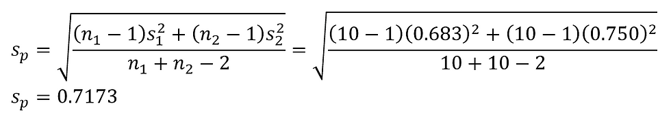
Plugging in the different values, we can then find the test statistics and its degree of freedom.

Looking at the t-table, we can see that the critical value at a 5% level of significance is -1.7341, meaning that the test statistics does fall into the rejection region. Thus, we reject our null hypothesis, concluding that there is significant evidence that the new machine is faster than the old machine.

---

Unpooled Variance

Awesome! Now that we learned the pooled t-test, let's take a look at the other scenario when the two standard deviations are dissimilar. Note that because the mathematics and theory behind are complicated for this case, so they're intentionally left out.

The assumptions that the two populations are independent and normal (or large sample size) should still hold true. The only difference here is that the assumption of equal variance is no longer valid.

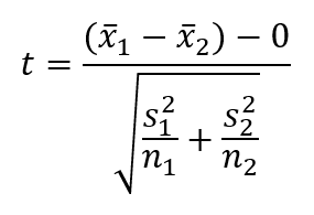
Under these assumptions, the formula for the t-test statistics would become:

With degrees of freedom:

Again, the math behind this derivation is complicated and goes beyond the scope of this tutorial, so just remember that this is the final simplified formula.

Confidence Interval

Given the formula, we would also know the formula to the confidence interval:

Example

Just like how we demonstrated an example for the pooled t-test, let's also try an example here with unpooled variance. (Example retrieved from Penn State Stats Online)

Independent random samples of 17 sophomores and 13 juniors attending a large university yield the following data on grade point averages:

Screenshot from Penn State Online

At the 5% significance level, does the data provide sufficient evidence to conclude that the mean GPAs of sophomores and juniors at the university differ?

We begin by checking the assumptions. The two populations are independent since sophomores and juniors are two distinctive groups. The sample sizes are small (n<30) and there is no indication that the two populations are normal. But for the sake of this example, let's first assume that they are normal. Next, we need to determine whether we should use the pooled t-test or the non-pool t-test. The standard deviation for the two samples is 0.520 and 0.3093, respectively. Considering that the sample sizes are both very small and that the standard deviations are quite different, let's use a non-pooled t-test in this scenario.

We define the hypotheses first like always.

And then we proceed to calculate the t-test statistics and its degree of freedom using a non-pooled variance. Give this question a shot. In the end, you should derive a t-statistics of -0.92 with a degree of freedom 26.

Comparing the t-test statistics to the critical value (5% level of significance), we can determine that the t-test statistics do not fall within the rejection region. We do not reject the null hypothesis and conclude that there is insufficient evidence that the mean GPA of sophomores and juniors are different.

---

Conclusion

Wow! We covered quite a lot of content in this story. We discussed how to conduct statistical tests that compare two means. It's important that you always check the assumptions, because we learned that by checking the difference between the two standard deviations, we would perform either a pooled t-test or a non-pooled t-test. The other assumptions on independence and normality are also equally important as highlighted in the previous story, so do not ignore them! After you determine which test to conduct, the remaining procedures on hypothesis testing or confidence interval estimation are all just the same. In our next story, we will discuss about inferences for paired means, or in other words, when two samples are not independent. Stay tuned!