How Do You Compare Two Population Proportions?

If you have been following the previous lessons on inferential statistics (sampling distribution, CI estimation and hypothesis testing for both sample mean and sample proportion), you should notice that we've been focusing on only one single variable. For example, for hypothesis testing for the sample mean, our objective is to test a population mean, which only concerns one numerical variable. This is referred to as univariate data.

In this story, we'll be dealing with situations that involve two variables, also referred to as bivariate data. Here are the two cases in which we will consider:

1. Categorical (explanatory) and categorical (response)

2. Categorical (explanatory) and numerical (response)

The first case involves comparing two independent proportions.

• An example would be measuring sex (explanatory) and whether the person smokes or not (response).

The second case involves comparing two independent means.

• An example would be measuring education level (explanatory) and GPA (response).

Before you proceed, I strongly recommend you to study the following chapters if you haven't:

• Statistics 9: Sampling Distribution Clearly Explained!

• Statistics 10: Confidence Interval Estimation

• Statistics 12: The Intuition of Hypothesis Testing

• Statistics 13: Hypothesis Testing (Z-test)

• Statistics 15: Inference about Proportion

• Statistics 16: Hypothesis Testing (Proportion)

All of these stories build up your fundamentals of inferential statistics, which is a strict prerequisite for this story.

---

The Idea

When we deal with two population parameters, we consider the difference between the two population parameters:

The idea is that when the difference is equal to zero, then the two population parameters are equal. But let's not get too ahead of ourselves. In inferential statistics, we typically deal with sample statistics and sample statistics are not represented by a single value. A sample mean, for example, can be different based on different samples. Therefore, sample statistics are usually represented in distribution, also known as the sampling distribution (Study Statistics 9: Sampling Distribution if you don't remember).

So how do we find the difference between two distributions? Luckily, mathematicians have worked out the details for us:

Don't worry if this looks too complicated! We'll look into examples of this theory later. For now, just remember that this is what happens when you try to deduct two normal independent distributions. It forms a new normal distribution with the mentioned mean, variance and standard deviation.

---

Comparing Two Population Proportions

Ok, let's begin by considering the first case scenario, comparing two population proportions. This means that we are dealing with two categorical variables here. Let's look directly at an example. (example retrieved from Penn State online statistics notes)

Males and females were asked about what they would do if they received a $100 bill by mail, addressed to their neighbor, but wrongly delivered to them. Would they return it to their neighbor? Of the 69 males sampled, 52 said "yes" and of the 131 females sampled, 120 said "yes." Does the data indicate that the proportions that said "yes" are different for males and females?

Let's denote the male and female proportions who said "yes" first.

To indicate whether there is a difference in proportion, we have to see if their difference is equal to zero.

But it's not as simple as finding the difference between the two sample proportions, 120/131 and 52/69. Remember that sample proportions should not be seen as a single value, but as a distribution (the sampling distribution)! Therefore, we are essentially finding the difference between the two sampling distributions of sample proportions, one male and the other female.

Ok, now let's recall the theory mentioned earlier in the story.

Given this theory, if the two sampling distributions are normal and independent of each other, we can derive a new distribution that denotes the difference between the two distributions. Let's do that now!

First, we know for sure that the two distributions are independent. The male's decision does not impact the female's decision and vice versa. So we just have to make sure that the two sampling distributions are normal. Let's wind back to Statistics 15: Inference about Proportion and recall the conditions to check whether a sampling distribution of sample proportion is normal or not. The conditions are:

Let's quickly check these conditions for both the male and female sampling distributions.

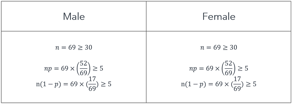
Because all of the conditions are satisfied, we can safely say that both sample proportions follow a normal distribution.

Ok, what next? In Statistics 15: Inference about Proportion, we also mentioned that we could derive the mean and standard deviation (standard error) of the sampling distribution for sample proportion.

We can apply these formulas to find the mean and standard deviation of the two sampling distributions.

Now that we have these values, we have all the components to find the new distribution that denotes the difference between the two sampling distributions. According to the theory:

Now that we have the mean and standard deviation of the new distribution that denotes the difference between the two sampling distributions, we can conduct our usual confidence interval estimation and hypothesis testing.

---

Confidence Interval Estimation

The formula structure for confidence interval remains unchanged. It is still:

In our current example, the formula becomes precisely:

Let's plug in the values and try to find the 95% confidence interval.

The result indicates that we are 95% confident that the difference in population proportions of males who said "yes" and females who said "yes" is between -0.02746 and -0.0502. Since the entire confidence interval is in the negative range, it appears that the proportion of females who said "yes" is higher than that of males.

---

Hypothesis Testing

Let's move on to hypothesis testing for two proportions. By now, you should know that we are mainly interested in whether the difference between the two proportions is zero or not. If the difference is zero, then the two proportions are equal. Therefore, our null hypothesis will always be:

Another way of looking at this null hypothesis is:

This is an interesting way of thinking about the null hypothesis because it essentially says that the two sample proportions are estimating the same proportion. Think of this proportion as p*. If this is true, then the sampling distribution of both sample proportions will be approximately:

So what would this new p* be? We can calculate p* by combining the two proportions.

Now, remember that in hypothesis testing, we always assume the null hypothesis to be true at first. This means that we do assume that the two sample proportions are estimating the same proportion, both of them being p*. The sampling distribution of the difference between the two sample proportions would therefore become:

Again, now that we have derived the mean and standard deviation of the sampling distribution, we can test to see if the difference between the sample proportions supports the assumption that the difference is zero. The formula for the Z value remains the same:

Plugging the formula into the current context and we have:

Note: The assumed value is zero because we made the assumption that the difference between the two proportions is zero.

After we found the Z test statistics, the critical value, rejection regions, p-value and decisions will all follow the same step as that of a typical hypothesis testing. Let's actually carry out the test, shall we? Let's perform the test at a 5% level of significance.

Step 1: Define Hypothesis

Step 2: Check Conditions

We already checked the conditions previously during confidence interval estimation, so I will not repeat them again.

Step 3: Compute Test Statistics

Step 4: Conclude

Because the test is a two-tailed test at a 5% level of significance, the critical values are ±1.96. The Z test statistic is clearly smaller than the lower critical value, meaning it falls into the rejection region. We can therefore conclude that there is enough evidence to suggest that the proportions of males and females who would return money are different.

---

Conclusion

Wow! That was a lot covered! In summary, this story discussed CI estimation and hypothesis testing for two proportions. This story shouldn't be too hard if you have a strong grasp of the sampling distribution, inferences about proportion and hypothesis testing. For those struggling, I strongly encourage you to go back and review those first. In the next story, we will move on to discuss the second case scenario where the response variable becomes numerical. In other words, we will be comparing two means instead.