How to Calculate Confidence Interval: A Quick Guide
- 2022年3月3日
- 讀畢需時 8 分鐘
已更新:2024年1月22日
In this story, we will go over the topic of the confidence interval. Mastering confidence interval requires a well-rounded understanding of sampling distribution. So, if you haven’t studied that, I strongly recommend you brief yourself with sampling distribution first (Statistics 9: Sampling Distribution Clearly Explained!). Without further ado, let’s begin!
Point Estimate
In the first chapter, we discussed the relationship between population and sample. To recap, we extract a small portion of data, our sample, to represent the entire population. Measures that describe the population are known as population parameters (eg. population mean), whereas measures that describe the sample are known as sample statistics (eg. sample mean). When the population parameter is unknown, we like to estimate it using the sample statistic. In proper terms, we say that sample statistics are point estimates of population parameters. Here are some examples of point estimates.

The question with point estimates is “how do we assess the accuracy and reliability of point estimates?”. We know from sampling distribution that there is a variance with sample statistics. Every time we select a different sample, the sample statistics will vary a bit (meaning the estimate for population parameters will also vary). So how accurate and reliable are these point estimates?
Let’s take a random sampling distribution as an example. Below, we have a distribution of the sample mean age.

Remember that a sampling distribution is composed of many sample means, meaning every single value in this sampling distribution is technically a point estimate by itself. Thus, the standard deviation of the sampling distribution (also known as the standard error if you recall from the last story) tells us how accurately the sample means estimate the true population mean.
As we try to ‘estimate’ the population mean, we will inevitably make an estimation error. (as evidenced by the standard error) Not only do we want to have an estimate for the population mean, but we also want to have an idea about the estimation error. This is where the notion of confidence interval comes in, by ‘expressing’ our estimate as an interval, so it also considers the estimation error.
By definition, the confidence interval is the range of values that’s likely to include a population value with a certain degree of confidence.
Let’s visualize the confidence interval with another example of a sampling distribution.

In the above sampling distribution, if the area under the curve from the interval [260, 340] covers 95% (so there is a probability of 0.95 that sample mean will be between 260 and 340), then that means we are 95% confident that the true population mean lies within the interval [260, 340]. The interval [260, 340] is the 95% confidence interval.
Ok, before we move on to learn how to calculate the confidence interval, try to digest what we just covered. It’s important that you understand the intuition behind confidence intervals.
Find Confidence Interval
To find a confidence interval, we must check one condition first. Is the sampling distribution normal? If the sampling distribution is normal, then it becomes easy for us to calculate the interval in which the area under the curve covers the confidence percentage. If the sampling distribution is not normal, then it’s technically not possible to calculate the confidence interval. To keep things simple, when the sampling distribution is not normal, we have to make the assumption that it is. (We don't directly assume the sampling distribution as normal. Instead, we assume the population distribution is normal, which makes the sampling distribution normal. We covered this in the last story as well.)
Here is a flow chart that guides us in calculating a confidence interval.

To the left of this chart, we see that the sampling distribution is normal (enclosed in orange below). Only one small section to the right (enclosed in blue below) is where sampling distribution is not normal. As previously mentioned, we must assume that the population distribution is normal (so that sampling distribution is also normal) if the variable falls into this section.

After we determine the normality of the sampling distribution, we have to check whether the population standard deviation is known or not.
When the population standard deviation is known, we can find the confidence interval using the Z-distribution.
When the population standard deviation is unknown, we can find the confidence interval using the t-distribution.
You might be familiar with the Z-distribution from Statistics 8: Standardization. A Z-distribution is another term for standard normal distribution, where the mean is 0 and the standard deviation is 1. A t-distribution is another distribution that is very similar to the Z-distribution, and we’ll talk more about it soon.
Let’s put our focus on the Z distribution first.
Confidence Interval for μ (σ known)
Okay, let’s reiterate the two conditions that we have to check for calculating a confidence interval.
Is sampling distribution normal?
Is population standard deviation σ known?
Remember the ways to check the normality of a sampling distribution? (Mentioned in Statistics 9: Sampling Distribution Clearly Explained!)
If the population distribution is normal, then the sampling distribution is also normal
If the population distribution is not normal but n >= 30, then sampling distribution is normal (by central limit theorem)
If the population distribution is not normal and n < 30, then we cannot be certain of the shape of the sampling distribution (so to find the confidence interval, we must assume the sampling distribution is normal)
Now let's assume population standard deviation is known in this case, which means our sampling distribution follows a Z-distribution. We can then find the confidence interval using the following formula:

Let’s clarify some notations in this formula.

Confusing? No worries! Let’s try to visualize this formula. Assume we want to find the 95% confidence interval. The sampling distribution is normal and the population standard deviation σ is also a known value (sampling distribution follows a Z-distribution). Because we know that the sampling distribution follows a Z-distribution, we can easily find the critical value of 1.96 and -1.96 using the Z-table (refer to the visualization below).

The critical value is a specific Z-value that marks the upper and lower boundary of the confidence interval. Note that the Z-value also marks the number of standard deviations from the mean value of the distribution. This means that the critical value of 1.96 can be interpreted as 1.96 standard deviations away from the mean of 0. Therefore, we can multiply our critical value by the standard deviation of the sampling distribution (the standard error) to derive the distance from the mean to either the upper or lower boundary of the confidence interval. This distance is also called the sampling error or margin of error.

In case you don’t recall from Statistics 9: Sampling Distribution Clearly Explained!, we can derive the standard deviation of the sampling distribution (the standard error) by dividing the square root of n by the population standard deviation. This is why we had to check that we knew the population standard deviation in advance.

Now go back and take a look at the formula again. Not so complicated after all right? That was a lot of terminology! Take some time to understand what we just discussed. If you’re having trouble, it might be because your understanding of sampling distribution isn’t strong enough.
Here is a sample question to strengthen what we just learned.
A random sample of 15 stocks traded on the Hang Seng Index showed the average shares traded to be 215,000. From past experience, it is believed that the population standard deviation of shares traded is 195,000, and the shares traded are very close to a normal distribution. Construct a 99% confidence interval for the average shares traded on the Hang Seng Index.
Step 1: Check your conditions
Since population distribution is normal, the sampling distribution is also normal. The population standard deviation (195,000) is also known, so we can use the Z-distribution to find the confidence interval.
Step 2: Calculate the confidence interval

Interpretations of Confidence Interval
After we calculated our confidence interval, we have to be careful in our interpretation. Based on our sample question, many people might interpret the confidence interval as:
There is a 99% chance that the unknown population mean will fall between 85351.88 and 344648.12.
This is the wrong interpretation! If you think about it, the unknown population mean is either in that interval or not; there is no probability associated with it. The correct way to interpret confidence interval is:
We are 99% confident that the population average number of shares traded on the Hang Seng Index is between 85351.88 and 344648.12.
Other Factors Affecting Interval Width
There are two main factors that affect the confidence interval, sample size n and the level of confidence. Let’s take a look at the formula of confidence interval again:

It becomes pretty clear that:


Confidence Interval for μ (σ unknown)
Up until now, we’ve discussed how we can calculate confidence interval given the condition that population standard deviation is known. The population standard deviation allows us to derive the standard error (standard deviation of sampling distribution) and so can use a Z-distribution to derive the confidence interval. What happens when the population standard deviation is unknown? In fact, in most cases, the population standard deviation will be unknown. In this case, we have to estimate the value using the sample standard deviation S. Here is the formula for sample standard deviation if you don't recall.

But there is a problem with using sample standard deviation in place of population standard deviation.

T-distribution
A t-distribution is very similar to that of a Z distribution (or a standard normal distribution), except its shape depends on the degrees of freedom. The degree of freedom for a t distribution is n-1. The larger the sample size, the t distribution becomes more similar to a standard normal distribution. Below, we can see that the smaller the sample size, the fatter the shape of the distribution. You can kind of see this as a penalty for a smaller sample size.

T-table
The Z distribution has a Z table, and so the t-distribution would also have a t-table, except it is not entirely the same as the Z table.
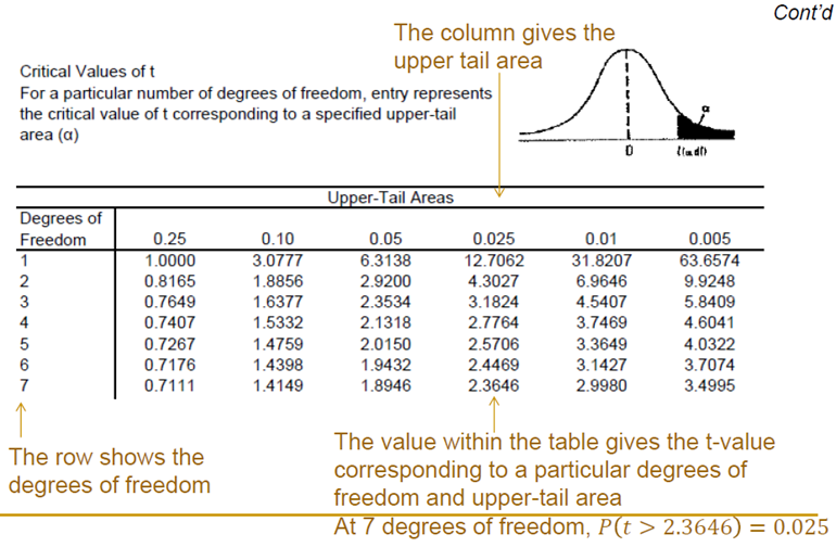
We can see that the t-table has degrees of freedom as its first column and upper-tail area as its first row. So the t-table actually gives you the t-value (similar to that of the Z-value) instead of the area under the curve (probability).
Now let’s try to find the confidence interval using a t-distribution (of course given that the population standard deviation is unknown).
We begin by checking the conditions required to find the confidence interval:
Population standard deviation is unknown
Population distribution is normal, thus sampling distribution is also normal, or
Population distribution is not normal but n>=30, thus sampling distribution is normal.
If all are satisfied, we can then use the following formula to find the confidence interval:

Perhaps it would be best illustrated by using an example.
The monthly salary of brokers is found to be normally distributed. A random sample of 25 brokers has a mean monthly salary of HKD 80K and a standard deviation of HKD 16K. Set up a 95% confidence interval estimation for the population mean.
Step 1: Check your conditions
The monthly salary of brokers (population) is normally distributed and so the sampling distribution is also normal. The population standard deviation, however, is unknown, so we must use a t-distribution to find the confidence interval.
Step 2: Calculate your confidence interval

Interpretation: We are 95% confident that the population mean monthly salary of brokers is between 73,396 HKD and 86,604 HKD
Conclusion
Wow! We covered quite a lot in this story! Let’s do a quick recap. By now you should understand the flow map for the confidence interval (below).

It’s crucial that you always check your conditions first before you dive into calculating the confidence interval.
First, we must make sure the sampling distribution is normal. If we cannot justify that the sampling distribution is normal, then we have to assume the population standard deviation is normal (so the sampling distribution is also normal). Stating this assumption is very important!
Then, depending on whether the population standard deviation is known or not, we will use either the Z-distribution or the t-distribution to find the confidence interval.
Finally, remember that confidence intervals are just estimates of population parameters expressed in the form of an interval (to consider the estimation error). We focused primarily on the parameter population mean in this story, but the concept of the confidence interval can be applied to every other population parameter.
In our next story, we will discuss how we can determine sample size in order to gain control over the sampling error. It is a topic closely connected with confidence interval, so keep on reading!


留言