What is Standardization and Why is it So Important in Statistics?

Extending from the previous story on distributions, this story will cover standardization. This is a very important concept to master before we advance, so take all the time you need for this story.

---

Standardization

In the previous story, we mentioned that we can use standardization to calculate the area under a normal distribution, which is also the probability. But let’s first let’s review the notation for a normal distribution.

You may recall that a normal distribution is denoted as:

The notation can be read as

Let’s see a few examples.

We have two normal distributions below. They’re each denoted as:

If you don’t remember from the previous story, the mean μ is the center of the normal distribution and the σ determines the spread of the distribution.

Now can you can see why finding the area under a normal curve can be such a hassle? The area distribution under the curve is different for the red curve and the blue curve, despite both of them being normal distributions.

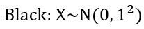
One way to fix this problem is to "standardize" the normal distributions, also known as the process of standardization. Standardization is the process that transforms any normal distribution into a standard normal distribution. A standard normal distribution is a normal distribution with a mean of 0 and a standard deviation of 1 (denoted below).

Any normal distribution can be standardized to a standard normal distribution. Let’s illustrate this below.

Both the red and blue curves can be "standardized" into the black curve, which is a standard normal distribution.

We can do so by applying the following formula to the red and blue distribution.

So how does this formula transform any normal distribution into a standard normal distribution? Let’s demonstrate this by "standardizing" the blue distribution.

Step 1: Focus on the current difference between the blue distribution and the black distribution (standard normal distribution).

Step 2: Deducting μ from the Xs of the blue distribution shifts the blue distribution such that it also has a μ of 0 (same center as the standard normal distribution).

Step 3: Then we divide the X values by σ, which changes the standard deviation to 1, completing the transformation from the original blue distribution to the standard normal distribution.

You can’t see the black curve in step 3 because it is overlapped with the blue curve. With two simple steps, we can transform any normal distribution into a standard normal distribution.

And now that we know we can transform any normal distribution into the standard normal distribution, we can put our focus on calculating the area under the standard normal distribution.

We can find the area under the curve of a standard normal distribution using the standardized normal table (also called the Z-table). The table looks something like this:

In the first column and row, we have the Z value. What is the Z value? Recall that in the standardization formula, we denote the result of the standardization by Z.

We’re essentially "standardizing" our original X variable to a Z variable. Based on the Z-value, we can then find the corresponding area under the curve to the left of the Z-value. Too confusing? Don’t worry! Everything will become clear with an example.

Assume variable X follows a normal distribution with a mean of 100 and a standard deviation of 10. What is the probability that X is greater than 110?

Below is the normal distribution of X. The probability that X is greater than 110 would be the area in red.

Now if we standardize this normal distribution, here’s the result.

Notice the mean is now 0 and the standard deviation is 1. During the standardization, 110 (the border of the original red area) is also standardized to 1.

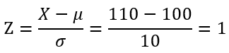
We can see that the border of the red area for the standardized distribution is now at 1. In other words, the red area under the curve is now P(Z>1). We can find this probability using the Z-table. We should look for the probability that corresponds to Z value 1.

The corresponding probability is 0.8413. But be extremely careful because the probability on the Z-table is usually the probability from -∞ up to the Z-value. This means that 0.8413 is P(Z<=1). (below)

Our target is to find P(Z>1), so we must remember to deduct P(Z<=1)=0.8413 from 1. In case you forgot, the total area under a distribution will always be 1.

The probability that the Z value is greater than 1 in a standard normal distribution is 0.1587. But don’t forget that this is the same as finding the probability that the X value is greater than 110 in the original distribution (when the mean is 100 and the std is 10).

Final Answer: The probability that X is greater than 110 in a normal distribution with mean 100 and standard deviation 10 is 0.1587.

This is the logic behind finding the area under a normal curve (probability) using standardization. Once you understand this, you can write out the equations to answer swiftly. Below is the proper work that you need to show for the same example we just discussed.

Quick Recap

Ok, before we conclude, let's quickly recap standardization.

1. Any normal distribution can be standardized into the standard normal distribution

2. Therefore, we can focus on calculating the area under the curve of the standard normal distribution.

3. The area under the curve of the standard normal distribution can be calculated using the Z-table.

4. Be aware that the Z-table displays the area under the curve to the LEFT of the Z-value.

---

Conclusion

Hooray! We just covered standardization and how it allows us to calculate the area under a curve. This is a very important topic, so take all the time you need to truly understand standardization. In our next story, we will step into sampling distribution, which is arguably just as important. Let's go!!!