The t-test 🧋

Note: This story is an extension of Statistics 13: Hypothesis Testing (Z-test), so a lot of details about Hypothesis Testing that have already been covered will not be repeated.

The t-test is very much like the Z test with some slight differences. In the last story, we were able to summarize hypothesis testing into four simple steps.

1. Define Hypotheses

2. Check your conditions (determine to use Z test or t-test)

3. Compute test statistics (to compare to the critical value in the critical value approach)

4. Conclude

In the t-test, step 1 is no different from the Z test. Given the scenario, you define the appropriate hypotheses that you want to test. It is in step 2 where things become a little bit different, so let's start there.

Step 2: Check your Conditions

You may recall the reason we check conditions is to ensure that the correct type of test is conducted. For hypothesis testing for the population mean μ, we can either do a Z test or a t-test. The following flow map guides us in determining which test to use.

We know from the previous story that if the sampling distribution, after standardization, follows a t-distribution, we have to perform a t-test. Based on the flow map above, this means that if the population standard deviation σ is unknown, we have to use a t-test. You should notice by now that 'whether population standard deviation σ is known' will determine whether we should use a Z test or a t-test.

Since we're focusing on the t-test in this story, we'll be assuming that the population standard deviation σ is unknown.

Step 3: Compute test statistics (and critical value)

In the t-test, we compute the t-test statistics instead of the Z test statistics (in the Z test). Both of these test statistics are the standardized value of the sample statistics (sample mean in this case). Let's compare to see how the formulas of the t-test statistic and the Z-test statistics are different.

The primary difference in the calculation is in the use of standard deviation. The Z test statistics use the population standard deviation (because it is known). The t-test uses the sample standard deviation to replace the unknown population standard deviation. The problem with using S in place of σ is that the standardized distribution will follow a t-distribution (hence the use of notation t) with degrees of freedom n-1. I wrote an entire story that digs into the depth of the differences between the Z Distribution and the t-distribution, so I recommend you to take a look at that first as well.

Anyways, the main point here is that there is a slight difference in the calculation of the test statistics. After we find the test statistic, we want to compare it with the critical value, and depending on the type of test, we want to determine whether it falls into the rejection region or not. The calculation for the critical value in a t-test would also be slightly different. Let's again compare the calculation for critical value in a Z test and in a t-test.

Critical Value in a Z test

Critical Value in a t-test

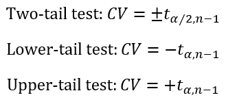
We can see that, except for the difference in notation (Z and t), the critical value in the t-test also depends on the degrees of freedom n-1. The other obvious difference is

that you would derive the critical value in a Z test from the Z-table, whereas you would derive the critical value in a t-test from a t-table.

Step 4: Conclude

After we are able to find the test statistic and the critical value, the decision to 'reject' or 'don't reject' will also be no different from the Z test. We check to see whether the test statistic falls into the rejection region and then make the corresponding conclusion.

Summary

Let's quickly sum up the main differences between the Z test and the t-test.

Z test	t-test
Use when population standard deviation σ is known	Use when population standard deviation σ is unknown
Critical value derived from the Z table and is dependent on the level of significance α	Critical value derived from the t-table and is dependent on the level of significance α and degrees of freedom n-1
​Z test statistics uses population standard deviation σ	t-test statistics uses sample standard deviation S

Perhaps it's best to demonstrate the t-test by looking into an example. Here we go!

Example:

A manufacturer of chocolate candies uses machines to package candies as they move along a filling line. Although the packages are labeled as 8 ounces, the company wants the packages to contain a mean of 8.17 ounces so that virtually none of the packages contain less than 8 ounces. A sample of 50 packages is selected periodically, and the packaging process is stopped if there is evidence that the mean amount packaged is different from 8.17 ounces. Suppose that in a particular sample of 50 packages, the mean amount dispensed is 8.159 ounces, with a sample standard deviation of 0.051 ounces.​

Is there evidence that the population mean amount is different from 8.17 ounces? (use a 0.05 level of significance)​

Step 1: Define Hypotheses

The question is asking us whether there is evidence that the population mean amount is DIFFERENT from 8.17 ounces. From this statement alone, we can define our two hypotheses as:

Step 2: Check your conditions

We have to check our conditions to make sure that we are using the right test. The two conditions are 1) make sure sampling distribution is normal and 2) check whether population standard deviation σ is given or not.

1. n=50 which is greater than 30, so according to the central limit theorem, the sampling distribution is normal

2. The population standard deviation σ is unknown (we only know the sample standard deviation S at 0.051 ounces), which means we have to use a t-test.

Step 3: Compute test statistics (and critical value)

Now that we've determined that we want to use a t-test, let's calculate the t-test statistic and compare it to the critical value. The question tells us that we have a sample mean of 8.159 ounces. We can find the t-test statistic by standardizing this 8.159 ounces.

Next, let's find the critical value. We have a two-tail test, so we must remember to use α/2.

Now let's visualize what we have at this point.

The white area on the two sides of the distribution is the rejection region. Since -1.5251 is less than -2.0096, the test statistic does not fall into the rejection region.

Step 4: Conclude

Since the test statistic does not fall into the rejection region, we do not reject at a level of significance α=0.05. This means there is insufficient evidence that the population mean amount is different from 8.17 ounces.

---

Finding the P-value in a t-test

Finding the p-value in a t-test is particularly tricky. In case you don't know what the p-value is (we covered this in the previous story as well), the p-value is the probability of obtaining a more extreme test statistic, given H0 is true. The condition 'given H0 is true' simply refers to the distribution (the distribution is built based on the assumption that H0 is true). In our example, since we're dealing with a two-tail test, the p-value would also lie on both ends of the distribution, despite the test statistic -1.5251 being only on the lower tail.

To visualize the p-value in our example, it would be the area in white on the two ends of the t-distribution (with df=49) below.

We can find the upper-tail area by referring to the t-table. We focus only on the row with degrees of freedom 49 and we see that the row consists of only six t-values. This means 1.5251 is likely not going to be one of the values. In this case, 1.5251 lies in between 1.2991 and 1.6766, which corresponds to upper tail areas 0.10 and 0.05, respectively. This means our upper-tail area will also lie between 0.05 and 0.10. We are not able to derive an exact value using the t-table, so we represent the upper-tail area in the form of an interval, indicating that this is the range in which the value falls in.

If the upper-tail area is (0.05, 0.10), this means that the sum of the white region (our p-value) would be (0.05, 0.10) times 2 because the t-distribution is symmetric.

So yeah! In a t-test, we represent our p-value in the form of an interval because the t-table is not detailed enough. To find the exact p-value, you may need to resort to other computer software or calculators.

---

Conclusion

Not too difficult right? This story acknowledges the main differences between a t-test and a Z test. If you have trouble understanding this story, it could be because you lacked the fundamental understanding mentioned in the previous stories.

• Statistic 12: The Intuition of Hypothesis Testing

• Statistic 13: Hypothesis Testing (Z-test)

In our next story, we will move on to a new topic about proportions.