Is A statistically different from B?

In this story, we will go through the critical steps of performing hypothesis testing. In case you haven't gone through Statistics 12: The Intuition of Hypothesis Testing, I strongly recommend you do so first. You'll have a much better understanding of what we'll be doing in this story.

---

Step 1: Define your Hypotheses

For every hypothesis testing, we define two hypotheses: the Null Hypothesis (H0) and the Alternative Hypothesis (H1).

• The null hypothesis H0 is the assumption about the population parameter that we assume to be true at the start.

• The alternative hypothesis H1, on the other hand, is just the opposite of H0.

Let's demonstrate this by using the example of GPA from the previous story. CityU claims that the population mean GPA is 2.8 and we want to perform hypothesis testing to test whether the claim is true or not. To test this claim, we would have to assume it to be true first (μ=2.8). Notice this happens to match with the definition of the null hypothesis, and so our null hypothesis would be μ=2.8.

The alternative hypothesis would be the opposite of H0, and so we can define H1 as:

In the end, we will conclude one of the two hypotheses, either that the true population mean is what CityU claims to be 2.8 (H0) or that the true population mean is not what CityU claims to be 2.8 (H1). We will decide to either "reject the null hypothesis" or "don't reject the null hypothesis".

Note: The convention is we either "reject H0" or "don't reject H0". We never say we "accept H1".

When do we reject?

If you have read Statistics 12: The Intuition of Hypothesis Testing, you would know that we should reject the null hypothesis when the likelihood of obtaining the sample statistics is too low. But how low? To understand when we should reject, we must understand the concept of the rejection region.

The rejection region is the area containing the unlikely values of test statistics, given the null hypothesis is true. In other words, if the sample statistics fall into the rejection region, we should reject the null hypothesis. There are two crucial characteristics of the rejection region that we must understand:

• the size of the rejection region depends on the level of significance α

• the location of the rejection region depends on the type of test (two-tail test, lower-tail test, or upper-tail test)

The following illustration should clear things up a bit:

First of all, it becomes very clear to see how the rejection region is located on different sides of the distribution for different types of tests. All of these locations make logical sense. Take the two-tail test as an example. In a two-tail test, we are testing to see if the true population mean GPA is 2.8 or not. If we were to reject the null hypothesis, we would conclude that the true population mean GPA is not 2.8, but we won't be able to tell whether the population mean is greater than 2.8 or less than 2.8. Therefore, the rejection region falls on both sides.

• If the sample mean is significantly greater than the assumed population mean, then we would have to reject the null hypothesis

• If the sample mean is significantly less than the assumed population mean, then we would also have to reject the null hypothesis.

This is why the rejection region is on both sides for the two-tail test. The same logic applies to the two one-tail tests.

Regarding the area of the rejection region, even though the rejection region for the two-tail test resides on two sides, the total area of the rejection region remains to be α. Each side will be α/2.

You'll also notice that the boundary of the rejection region is called critical value. Therefore, to see whether the sample mean falls into the rejection region, we have to compare it to the critical value.

Step 2: Check your Conditions

There are many different types of tests for hypothesis testing, so we must ensure that we are using the right one. In hypothesis testing for population mean μ, we can either do a Z test or a t-test. To determine which one to use, the following flow map will help guide us.

You might recall this flow map from Statistics 10: Confidence Interval Estimation. They are the exact same map because we are standardizing the sampling distribution in both cases. It is important to know whether the sampling distribution, after standardization, will follow a Z distribution or a t-distribution.

• If the standardized sampling distribution follows a Z distribution, then we have to do a Z test

• If the standardized sampling distribution follows a t distribution, then we have to do a t-test

For more details on the difference between a Z distribution and a t-distribution, this post Z Distribution and t-distribution should be a great read.

Step 3: Compute Test Statistics

After we check our conditions and decide which test to use, we want to compute the test statistics. In hypothesis testing for population mean μ, the test statistics refers to the standardized sample mean, the Z-value (for a Z test), or the t-value (for a t-test) of the sample mean. Let's try to visualize what I mean with a Z test first.

In the previous example on GPA, we defined our hypotheses as:

Remember we assumed that CityU's claim is true (μ=2.8) and now let's also make the assumption that the population standard deviation for GPA is 0.5 (σ=0.5). Let's also assume that we are taking a sample size of n=36. These assumptions are in place such that the conditions (in Step 2: Check your Conditions) for a Z-test are met.

• Since n >= 30, the sampling distribution is normal based on the central limit theorem

• Since population standard deviation σ is known, the standardized sampling distribution will follow a Z distribution, which means we use a Z test.

Given these assumptions, we can also easily derive the mean and standard deviation of the sampling distribution (of sample mean GPA).

Remember that we are conducting a two-tail test, so the rejection region will fall on both ends of the distribution. The area of the rejection region is dependent on the level of significance α, so let's assume α=0.05.

Note that the illustration above is just for you to visualize what's going on. It is not completely accurate. The two critical values are not located where it seems to be in the illustration. We only know for sure the area of the two rejection regions, each accounting for

α/2=0.025. To find the critical value, we must apply standardization to the sampling distribution.

If you need a recall on standardization, you may visit Statistics 8: Standardization. Since population standard deviation σ is known, the sampling distribution gets standardized to a Z distribution (the same as a standard normal distribution with μ=0 and σ=1). We can then refer to the Z-table to find the critical value.

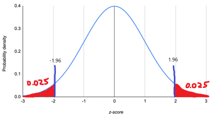
We find that the critical values are -1.96 and 1.96. This means that if the Z test statistics (the standardized sample mean) is less than -1.96 or greater than 1.96, it falls into the rejection region (which would lead to a rejection of H0).

Let's take a sample mean of 3.0 as an example. To see whether a sample mean of 3.0 will fall into the rejection region, we have to standardize this value so that it can be compared to the critical value (-1.96 and 1.96). The resulting standardized value is our Z test statistics.

Step 4: Conclude

Since 2.4 is greater than 1.96, the test statistics do fall into the rejection region. Therefore, we would reject H0 and conclude that there is sufficient evidence that H1 (true population mean is not 2.8) is true.

---

Critical Value Approach and P-value Approach

In the example demonstrated just now, we were able to arrive at a conclusion by comparing the critical value (1.96) to the test statistics (2.4). This method is called the critical value approach. But there's actually another approach that will do just as good of a job, the p-value approach. In the p-value approach, we compare the level of significance α to the p-value.

P-value - the probability of observing more extreme test statistics, given H0 is true

Let's explain the p-value approach through some visualizations. Using the same previous example, we can easily compare the level of significance α (red area) to the p-value (green shaded area).

Not too hard to understand right? The p-value, area in green, is the probability of observing a more extreme test statistic, which is 2.4, given H0 is true. The condition 'given H0 is true' simply refers to the distribution (the distribution is built based on the assumption that H0 is true). In this case, since we are dealing with a two-tail test, we have to account for the green area on both sides (P(Z<-2.4) and P(Z>2.4)). Although our test statistic is only 2.4, if we only compare the green area on the right to the level of significance α (red area on both sides), it wouldn't be a fair comparison.

The p-value here can be easily calculated using the Z table.

Note: In a one-tail test, the p-value would only be on one side of the distribution, so there would be no need to multiply two.

Since the p-value (0.0164) is smaller than the level of significance α=0.05, the test statistics must fall in the rejection region, and so we would make the same decision to reject H0. The benefit of using the p-value approach is that once you find the p-value, you can compare it to any level of significance you desire. Take the p-value=0.0164 that we just calculated as an example. If α=0.01 instead, we could quickly conclude to not reject H0 because the p-value is greater than α=0.01. There's no need to make another calculation. Easy!

---

Conclusion

Amazing! We just conducted a Z test from zero to hero! Let's quickly recap the main steps.

1. Define hypotheses

2. Check conditions (Z test or t-test)

3. Compute test statistics (compare to the critical value in the critical value approach)

4. Conclude

Not too complicated right? Let's end this story for now, but we're not done yet! Remember there's also a t-test that we've yet to discuss. In the next story, we will go over the t-test!